library(tidyverse) #loads package
library(ggplot2)
library(DescTools)

mma <- read_csv("mma.csv") #loads dataMMA Fight Decisions
Variable types
Chi-square test (2x2)
Fisher Exact test
Chi-square test (rxc)
Mosaic plots
Exploring MMA fight decisions by weight category
Welcome video
An interview with Nate Latshaw of LiteralFightNerd.com
Introduction
In this module, you will be analyzing data from mixed martial arts (MMA) fights in order to determine if the weight class of the fighters is related to the type of decision that ended the fight.
We speculate that knockouts are more likely for heavier weights. The difference, if it exists, has potential implications for marketing fights: are knockouts more exciting or would the MMA prefer longer fights?
Getting started: MMA data
The first step to any analysis in R is to load necessary packages and data.
You can think of packages like apps on your phone; they extend the functionality and give you access to many more features beyond what comes in the “base package”.
Running the following code will load the tidyverse, ggplot2, other packages, and the mma data we will be using in this lab.
TIP: As you follow along in the lab, you should run each corresponding code chunk in your .qmd document. To “Run” a code chunk, you can press the green “Play” button in the top right corner of the code chunk in your .qmd. You can also place your cursor anywhere in the line(s) of code you want to run and press “command + return” (Mac) or “Ctrl + Enter” (Windows).
TIP: Using a hashtag in R allows you to add comments to your code (in plain English). Data scientists often use comments to explain what each piece of the code is doing.
We can use the glimpse() function to get a quick look (errr.. glimpse) at our mma data. The glimpse code provides the number of observations (Rows) and the number of variables (Columns) in the dataset. The “Rows” and “Columns” are referred to as the dimensions of the dataset. It also shows us the names of the variables (date, day, …, wtClass) and the first few observations for each variable (e.g. the first two fights in the dataset took place on December 4, 2010 and May 15, 2010).
glimpse(mma)Rows: 28,771
Columns: 20
$ date <chr> "12/4/10", "5/15/10", "6/12/09", "1/23/09", "3/25/22", …
$ month <dbl> 12, 5, 6, 1, 3, 4, 2, 5, 1, 9, 1, 8, 6, 12, 2, 3, 1, 12…
$ year <dbl> 2010, 2010, 2009, 2009, 2022, 2021, 2021, 2018, 2018, 2…
$ event <chr> "Strikeforce: Henderson vs. Babalu 2", "Strikeforce: He…
$ championship <lgl> FALSE, FALSE, FALSE, FALSE, FALSE, FALSE, FALSE, FALSE,…
$ decision <chr> "Decision - Unanimous", "Submission", "TKO", "Unanimous…
$ decision_group <chr> "Decision", "Submission", "KO/TKO", "Decision", "KO/TKO…
$ round <chr> "3", "1", "2", "3", "1", "3", "3", "2", "1", "3", "1", …
$ time <time> 05:00:00, 00:56:00, 01:47:00, 05:00:00, 01:37:00, 05:0…
$ p1_result <chr> "L", "W", "L", "L", "L", "L", "W", "L", "L", "W", "L", …
$ p1_id <dbl> 2504991, 2504991, 2504991, 2504991, 4239497, 4239497, 4…
$ p1_name <chr> "Aaron, Tom", "Aaron, Tom", "Aaron, Tom", "Aaron, Tom",…
$ p1_country <chr> "USA", "USA", "USA", "USA", "ESP", "ESP", "ESP", "ESP",…
$ p1_sex <chr> "M", "M", "M", "M", "M", "M", "M", "M", "M", "M", "M", …
$ p2_result <chr> "W", "L", "W", "W", "W", "W", "L", "W", "W", "L", "W", …
$ p2_id <dbl> 2504993, 2504992, 2504956, 2514253, 5078428, 4236955, 4…
$ p2_name <chr> "Ricehouse, Matt", "Steenberg, Eric", "Voelker, Bobby",…
$ p2_country <chr> "USA", "CAN", "USA", "USA", "BRA", "USA", "ENG", "USA",…
$ p2_sex <chr> "M", "M", "M", "M", "M", "M", "M", "M", "M", "M", "M", …
$ wtClass <chr> "Lightweight", "Catchweight", "Welterweight", "Lightwei…ERROR? Did you get a error message that says could not find function "glimpse"? This means you need to load the tidyverse package. You can do this by running the code library(tidyverse) from the previous code chunk. A shortcut is to hit the “fast-forward” button (next to the “Play” button in your code chunk), which will run all code chunks above your current one.
MMA lingo
Before proceeding with any analysis, let’s make sure we know some MMA lingo in order to understand what information is contained in each variable (column) in our dataset.
The basics
- Fights consist of rounds (typically 3).
- Fights may end early due to:
- A submission: one fighter “taps out” or concedes.
- Knockout (KO) or Technical knockout (TKO) (the referee stops the fight).
- If a fight is not stopped early, then the winner is determined by judges (known as a decision).
- The decision could be unanimous (U) if all judges agree, or split (S) if not all judges agree.
- Championship fights are those which determine who is the champion of a given weight class.
- Fighters are in different weight classes and may only fight in their own class or higher weight classes as described below.
Totally new to MMA? See this site: INTRODUCTION TO MMA
Variable descriptions
The data used in the following examples comes from MMA fights posted on ESPN.com in 2023. The dataset does not include every possible fight, but it contains most fights available on ESPN from 1991 through 2023. Each row includes general information about the fight, such as the date, event name, and whether the fight was a championship bout. The dataset also includes fighter-specific information for each participant. Variables beginning with p1 refer to the first fighter, while variables beginning with p2 refer to the second fighter.
Show variable descriptions
| Variable | Definition | Example_Values |
|---|---|---|
| date | date of the event (mdy) | 10/12/2023 |
| month | month of the event | 10 |
| year | year of the event | 2023 |
| event | name of the event | UFC 1: The Beginning |
| championship | is the event a championship event | TRUE/FALSE |
| decision | fight result | TKO (Injury) |
| decision_group | aggregated groups of decision variable | KO/TKO |
| round | how many rounds the fight lasted | 3 |
| time | time the fight ended | 4:42 |
| p1_result | result of the fight for fighter 1(2) | W |
| p1_id | a unique ID for fighter 1(2) | 2354059 |
| p1_name | full name of fighter 1(2) | Shamrock, Ken |
| p1_country | home country of fighter 1(2) | USA |
| p1_sex | sex of fighter 1(2) | M |
| wtClass | aggregated groups of Weight Class | Heavyweight |
TIP: Type your answers to each exercise in the .qmd document.
TIP: To determine if a variable is categorical, read more about variable types here.
Viewing your data
You saw that glimpse() is one way to get a quick look at your data. Often, you’ll want to view your whole dataset. There are two ways to do this:
TIP: Recall that RStudio is split into four quadrants: Source (upper left), Environment (upper right), Console (bottom left), and Files/Plots/Packages/Help/Viewer (bottom right)
- type
View(mma)in your Console and then click return/Enter on your keyboard. - OR, in your Environment tab, double click the name of the dataset you want to view.
This will open up your data in a new viewer tab so that you can view it like a spreadsheet (like Google Sheets or Excel*). Once open, you can sort the data by clicking on a column.
*Unlike Google Sheets or Excel, however, you won’t be able to edit the data directly in the spreadsheet.
TIP: Type your answers to each exercise in the .qmd document.
TIP: To determine if a variable is categorical, read more about variable types here.
TIP: When viewing the data, clicking on a column once will sort the data according to that variable in ascending order; clicking twice will sort in descending order.
Example 1: Chi-square Test
We return to the first of our two research questions:
Notice that the two variables involved are wtClass and decision_group and both are categorical. For this research question, we have 2 categories for the wtClass variable (heavyweight and middleweight) and will have 2 decision_group categories (decision or KO/TKO/Submission). Data of this sort leads us to use of the chi-square test.
Chi-square Test Overview
The chi-square test is a test used to determine if there is a significant association between two categorical variables. It compares the observed frequencies of the different categories with the expected independent frequencies. The hypotheses involved are:
- \(H_0:\) there is no assocation between the two variables (null hypothesis)
- \(H_a:\) there is an assocation between the two variables (alternative hypothesis)
The hypotheses can also be thought of in terms of proportions with the null hypothesis that the proportions in categories of one variable are the same across categories of the second variable.
We will use the MMA data to explore the test and determine if, since the year 2020, fighter weight class and the decision of a fight are associated. In order to perform the analyis we will produce a “contingency table” displaying the data (note: To perform a chi-square test in many software packages, it is often not necessary to format the data into a contingency table. Many packages can take data from a standard rectangular data table and pass it through a chi-square function. R allows for either.). Additionally, we will illustrate how to present the data in a more visual format.
Preparing the data
We first select the variables of interest, and “filter” the data to the categories we wish to compare and the years of interest.
# Select, filter, and prepare relevant data for analysis
data1 <- mma |>
  select(year, wtClass, decision_group) |>
  filter(year >= 2020) |>
  filter(wtClass == "Middleweight" | wtClass == "Heavyweight") |>
  mutate(decision = if_else(decision_group == "Decision", "Decision",
"KO/TKO/Submission"))TIP: in logical expressions, a double equal sign is used “==”.
TIP: in logical expressions, “|” is “OR”
TIP: mutate is a dplyr function that allows us to create new variables.
TIP: if_else returns the first value listed (“Decision”) if the logical expression is true, otherwise it returns the second value listed (“KO/TKO/Submission”)
View the “data1” data frame and confirm that you understand what the code produced.
Visualizing the data: the contingency table
A contingency table rows (r) are categories of the first variable and columns (c) those of the second variable. The “r x c” table cells are the counts for each combination of categories. In our example, both variables have two categories so we have a “2x2” contingency table:
table(data1$wtClass, data1$decision )
               Decision KO/TKO/Submission
  Heavyweight       241               570
Middleweight 164 334TIP: select the variable from “data1” using a “$” followed by the name of the variable.
We see that among the heavyweight fights, 241 ended with a decision.
The R package “DescTools” we loaded includes a function that will add percentages (by row, column, or total) as well as the totals for rows/columns (known as “margins”) to the table.
PercTable(data1$wtClass, data1$decision, rfrq = "010",
                     margins = c(1,2))
                       Decision   KO/TKO/Submission   Sum

Heavyweight    freq         241                 570   811
               p.row      29.7%               70.3%     .

Middleweight   freq         164                 334   498
               p.row      32.9%               67.1%     .

Sum            freq         405                 904 1'309
               p.row      30.9%               69.1%     .
TIP: the rfrq option identifies which percentages to display. A “1” in the second position as in our example adds row percentages. Changing the first position to “1” would give total percentages and to the third position column percentages.
TIP: we provide a vector, c(), with values 1 (row) and 2 (column) of which margins to add to the table. If we input c(1) we would get only the row totals.
We added row percentages; notice that the percentages total to 100% for each row of the table, including for the column totals row.
Visualizing the data: Mosaic plot
A Mosaic plot visualizes the contingency table using rectangles with widths proportional to the counts for each category or combination of categories. In the plot below, the two “columns” represent the weight classes. We can see that more fights were heavyweight since the first column bars are wider.
We can compare the two groups by then looking at the percentages of fights ending in decision in each weight class proportional to the total number of fights in each weight class. The colors help in this determination as red means the fight ended in decision, blue KO/TKO/Submission.
mosaicplot(~ wtClass + decision , data = data1,
           main = "",
           ylab = "Decision",
           xlab = "Weight Class",
           color = c("tomato", "steelblue"))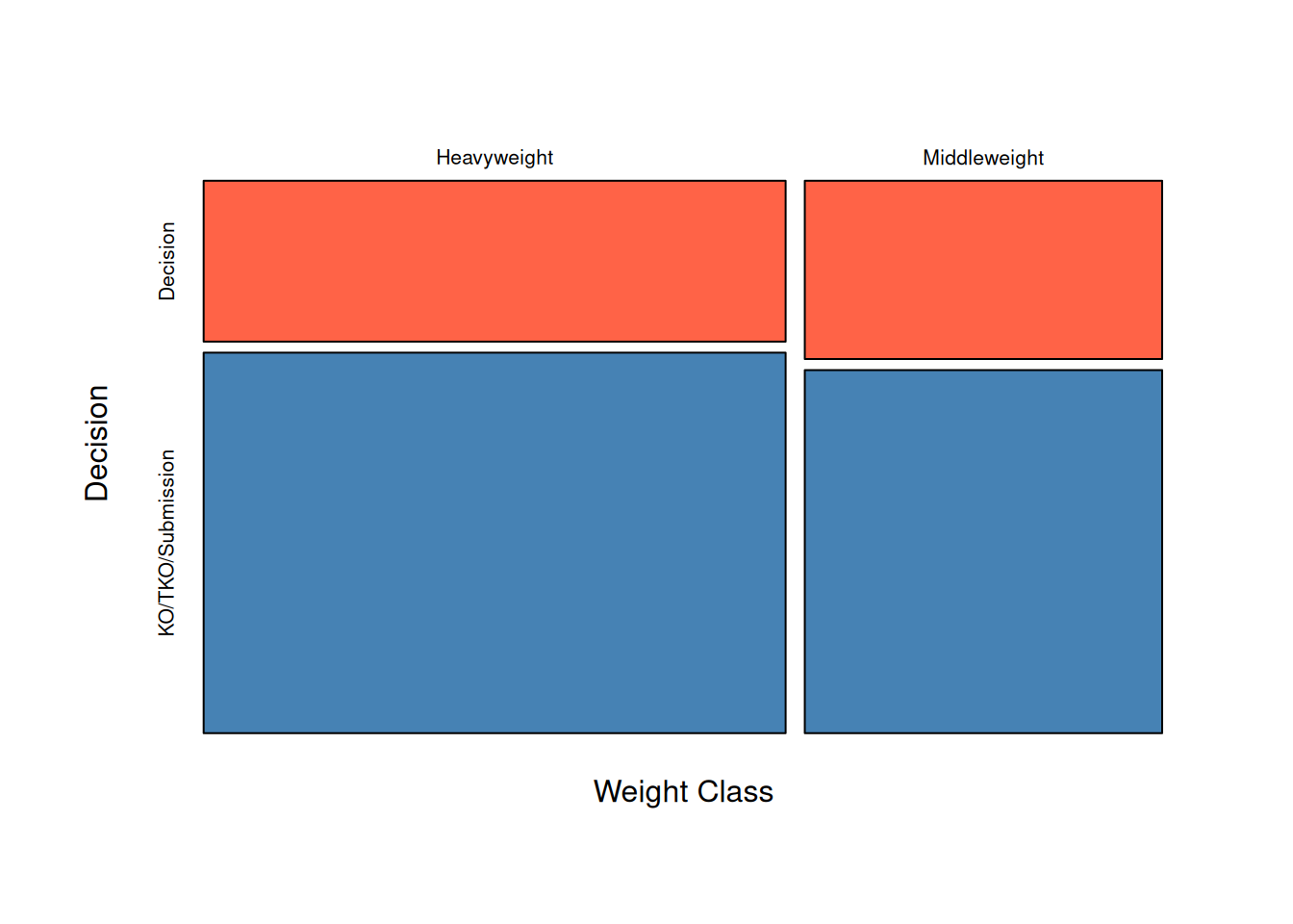
Conducting the Chi-square test
We first write the hypotheses presented earlier for our example:
- \(H_0:\) there is no assocation between weight class and whether the fight ended in a decision or not (null hypothesis)
- \(H_a:\) there is an assocation between weight class and whether the fight ended in a decision or not (alternative hypothesis)
The command “chisq.test” with the two variables as inputs performs the Chi-square test.
wt_decision.chisq <- chisq.test(data1$wtClass, data1$decision)TIP: save the test results into an object (here named “wt_decision.chisq”) in order to later extract all information produced.
Observed counts
We first confirm that the test has the correct data by extracting the “observed” values. These should be the same as in the contingency table.
wt_decision.chisq$observed data1$decision
data1$wtClass Decision KO/TKO/Submission
Heavyweight 241 570
Middleweight 164 334Expected counts
We next extract the “expected” values computed in order to perform the test. These are values that would be observed if the sample perfectly matched the proportions suggested in the null hypothesis - exactly the same proportions in the two decision categories for each weight class category (and vice versa). You will explore this in the next exercise.
wt_decision.chisq$expected data1$decision
data1$wtClass Decision KO/TKO/Submission
Heavyweight 250.9206 560.0794
Middleweight 154.0794 343.9206Test results
The observed counts are unlikely to exactly match the expected (this is a sample). However, if the null hypothesis is true we would anticipate the reasonably close agreement. The Chi-square test statistic, \(X^2\), measures how well they agree as:
\[X^2 = \sum \frac{(O-E)^2}{E}\] In this expression, the \(\sum\) symbol means “sum” or add. The terms added involve the observed (O) and expected (E) counts. In our case, there are 4 such quantities (one for each cell of the tables). For example, for the first cell (row 1, column 1) the quantity computed is:
\[\frac{(241-250.9206)^2}{250.9206} = 0.39\]
We calculate in similar fashion for the other three cells, and then sum (add) the four values. The resulting value, 1.3462, is given in the output from the test “X-squared”.
wt_decision.chisq
    Pearson's Chi-squared test with Yates' continuity correction

data:  data1$wtClass and data1$decision
X-squared = 1.3462, df = 1, p-value = 0.2459
If the observed perfectly matches the expected in all cells the \(X^2\) value would be 0. Of course, that is unlikely. However, if the null hypothesis is true, a smaller value is more likely. But how small is reasonable? Put another way, how large a value - reflecting big differences in the observed and expected - would make us question whether the null hypothesis is true?
We answer this question, statistically, by calculating the probability of obtaining a value of \(X^2\) of 1.3462 (our observed value) or greater assuming the null hypothesis is true. If the null hypothesis is true, the distribution of possible \(X^2\) values follows a \(\chi^2\) (“Chi-squared”) distribution. There is one parameter for this distribution, known as the “degrees of freedom” (df). For an r x c contingency table:
\[df = (r -1) \times (c-1)\]
Since \(r = c = 2\) in our example, \(df = (2-1) \times (2-1) = 1\).
Advanced note on df: One can think of the degrees of freedom for the Chi-square test as the number of “free cells” in the table considering the column and row totals as fixed. For example, the total for row 1 of our table (Heavyweight) is 811. Once we know the number in the first column of the row is 241, the second column value is no longer “free” - it must be 570. Thus, we have 2 - 1 = 1 df for the row. The column df are similar. The total df = 1 means only 1 cell is truly “free”; in other words, once we know a single cell of the 4 the other 3 are fixed. Use the example table to convince yourself this is true. The more df, or “free cells”, the greater uncertainty so the Chi-square distribution variability increases.
With the distribution defined, we can compute the probability. The output from R gives us the result as the p-value of 0.2459. If the null hypothesis is true, we have a probability of roughly 0.25 of obtaining observed/expected differences as great as observed in our sample.
Typically, the null hypothesis is “rejected” if the p-value is pretty small. A common cutoff is 0.05. Since our value is not that small, we cannot reject the null hypothesis.
Example 2: Larger tables (r x c) and Fisher’s Exact Test
We next turn to our second research question:
We will see that adding more categories (larger contingency tables) does not change the analysis process or implementation of the test. However, but in this case we will encounter an issue that requires a slight modification to the test known as Fisher’s exact test. Larger tables are more likely to require this version of the test due to smaller sample sizes in categories.
We first select the variables of interest, and “filter” the data to the categories we wish to compare and the years of interest.
# Select, filter, and prepare relevant data for analysis
data2 <- mma |>
filter(year == 2023) |>
select(year, wtClass, decision_group) |>
filter(wtClass == "Flyweight" |
wtClass == "Bantamweight" |
wtClass == "Strawweight" |
wtClass == "Atomweight" ) |>
mutate(decision = if_else(decision_group == "Decision", "Decision",
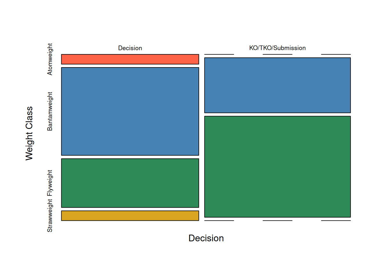
"KO/TKO/Submission"))We again visualize the data. We quickly observe that there is not a lot of data for the two lightest weight classes, atomweight and strawweight. In fact, neither category had a fight which did not end in decision.
mosaicplot(~ decision + wtClass, data = data2,
           main = "",
           xlab = "Decision",
           ylab = "Weight Class",
           color = c("tomato", "steelblue", "seagreen", "goldenrod"),
           las = 1, # rotate labels horizontal
           cex.axis = 0.8 # resize labels
           )
Chi-square Test
We can proceed with the Chi-square test. However, notice that R responds with a warning message. The test results are still produced and in this case we again cannot conclude evidence of an association (p = 0.1851). Notice the degrees of freedom for this example. With 4 weight class categories, we have \((4-1)\times(2-1) = 3\) degrees of freedom for the test.
wt_decision2.chisq <- chisq.test(data2$wtClass, data2$decision)Warning in chisq.test(data2$wtClass, data2$decision): Chi-squared approximation
may be incorrectwt_decision2.chisq
    Pearson's Chi-squared test

data:  data2$wtClass and data2$decision
X-squared = 4.8241, df = 3, p-value = 0.1851
The warning message is due to the assumption about expected cell counts. These values are well below the rule of thumb of five for both categories in the atomweight and strawweight classes.
wt_decision2.chisq$expected data2$decision
data2$wtClass Decision KO/TKO/Submission
Atomweight 0.4848485 0.5151515
Bantamweight 7.2727273 7.7272727
Flyweight 7.7575758 8.2424242
Strawweight 0.4848485 0.5151515Fisher Exact Test
When the assumption for the Chi-square test is not met, all is not lost! We can instead compute the p-value “exactly” using probability theory (the “hypergeometric” distribution is used, but we will omit the details).
The Fisher’s Exact Test assumes the row and column totals are fixed, then calculates the probability of a particular set of cell counts, then figures out all possible tables that could be constructed given the fixed totals, and calculates probabilities for each of these tables. The test determines which of these tables are extreme or more extreme than the table observed, and sums up the probabilities for the table seen and the more extreme tables to get the p-value.
The hypotheses for this test are the same as for the Chi-square test:
\(H_0\): Weight class and the fight decision are not associated.
\(H_a\): Weight class and the fight decision are associated.
The command is changed to “fisher.test”, but the general format of the command and output is unchanged.
wt_decision2.fisher <- fisher.test(data2$wtClass, data2$decision)
wt_decision2.fisher
    Fisher's Exact Test for Count Data

data:  data2$wtClass and data2$decision
p-value = 0.09378
alternative hypothesis: two.sided
The test returned a p-value of 0.09378. Our conclusion then after performing a Fisher’s Exact Test is again we do not have evidence to suggest that weight class and fight decision are associated (p = 0.09). In other words, we fail to reject our null hypothesis.
Notice that the p-value is changed by a fair amount in this example even though the conclusion is unchanged. The issue with the Chi-square assumption had an impact on the calculation in this case.
Case study 1: Exploring Results
When we have more categories (larger tables) the analysis is unchanged, but interpreting the results is more challenging. In this case study, we provide additional tools that can help identify which categories differ.
Examining the Sample
Below we select a larger sample of years and weight classes, and produce the output shown in previous examples. Use the output to answer the questions in the exercise.
# Select, filter, and prepare relevant data for analysis
data3 <- mma |>
  filter(year >= 2020) |>
  filter(wtClass %in% c("Strawweight", "Flyweight",
                              "Bantamweight", "Welterweight",
                              "Middleweight", "Heavyweight"))  |> select(year, wtClass, decision_group) |>
  mutate(decision = if_else(decision_group == "Decision",
                            "Decision",
"KO/TKO/Submission"))table(data3$wtClass, data3$decision)
               Decision KO/TKO/Submission
  Bantamweight      302               350
  Flyweight         248               263
  Heavyweight       241               570
  Middleweight      164               334
  Strawweight       123                80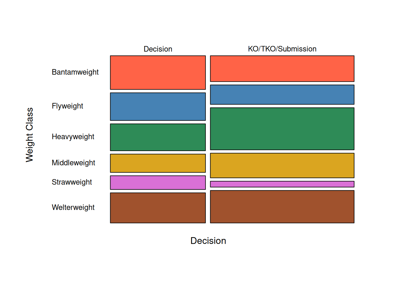
Welterweight 270 440mosaicplot(~ decision + wtClass, data = data3,
main = "",
xlab = "Decision",
ylab = "Weight Class",
color = c("tomato", "steelblue", "seagreen", "goldenrod", "orchid", "sienna"),
las = 1, # rotate labels horizontal
cex.axis = 0.8 # resize labels
)
Conducting the Test
Again, we provide output from a test. Use this to answer the exercise questions.
case1.chisq <- chisq.test(data3$wtClass, data3$decision)
case1.chisq$expected
data3$decision
data3$wtClass Decision KO/TKO/Submission
Bantamweight 259.64431 392.3557
Flyweight 203.49424 307.5058
Heavyweight 322.96248 488.0375
Middleweight 198.31728 299.6827
Strawweight 80.84018 122.1598
Welterweight 282.74151 427.2585case1.chisq
    Pearson's Chi-squared test

data:  data3$wtClass and data3$decision
X-squared = 109.58, df = 5, p-value < 2.2e-16Examining the Results
The statistically significant results from the test in this case study beg some questions.
- Which weight classes and which decision groups differ?
- We achieved statistical significance, but perhaps this is simply do to the very large sample size. Is there practical significance?
We can do an informal inspection of the observed and expected values (and also consider the visualization). We have already produced the observed (contingency) and expected tables. We add the row percentages below.
PercTable(data3$wtClass, data3$decision, rfrq = "010",
                     margins = c(1,2))
                       Decision   KO/TKO/Submission   Sum

Bantamweight   freq         302                 350   652
               p.row      46.3%               53.7%     .

Flyweight      freq         248                 263   511
               p.row      48.5%               51.5%     .

Heavyweight    freq         241                 570   811
               p.row      29.7%               70.3%     .

Middleweight   freq         164                 334   498
               p.row      32.9%               67.1%     .

Strawweight    freq         123                  80   203
               p.row      60.6%               39.4%     .

Welterweight   freq         270                 440   710
               p.row      38.0%               62.0%     .

Sum            freq       1'348               2'037 3'385
               p.row      39.8%               60.2%     .
Residuals
When we have a high number of rows and columns it is difficult to see if there are practical differences between certain cells. This may be achievable with a 2x2 table, but is much more difficult with larger tables. To help with this problem, we can calculate the Pearson standardized residuals which help identify cells we should investigate.
The formula for the Pearson residuals is:
\[\frac{(O-E)}{\sqrt(E)}\]
Notice this is the square root of the “contribution” of each cell to the overall test statistic \(X^2\). Essentially, the formula identifies cells that have large differences between observed and expected (the \((O-E)\) in the formula) but “standardizes” these differences (the \(sqrt(E)\) in the formula).
One way to think about the standardization is to consider a simple example. Suppose we have two cells with \(O-E = 2\). However, one cell has an expected count of 10 and the other an expected count of 1,000. In the first case, the \(O-E\) difference is 20% of the expected value. In the second, it is only 0.2% which is actually a small amount. The standardization basically puts these on the same scale.
Standardized residuals roughly follow a “normal distribution” which means we would expect approximately 95% of the values to between -2 and 2 and 99% between -3 and 3. Thus, values outside these ranges are somewhat unusual and cells that may contribute to a statistical association.
We can output the residuals from the Chi-square test in similar fashion to the expected counts:
case1.chisq$residuals data3$decision
data3$wtClass Decision KO/TKO/Submission
Bantamweight 2.6285868 -2.1383153
Flyweight 3.1198964 -2.5379882
Heavyweight -4.5607794 3.7101246
Middleweight -2.4368714 1.9823578
Strawweight 4.6890531 -3.8144733
Welterweight -0.7577501 0.6164182Case study 2: Putting it all together
Conclusion
Chi-square tests and associated analysis are useful for answering research questions that involve two categorical variables. In our examples, we explored the relationship between the type of MMA fight result and the weight classes using chi-square tests. We were interested in determining if, for example, fights at higher weight classes tend to have different outcome distributions compared to lower weight classes. For example, one might speculate that the heavier weight class fights are less likely to “go the distance” due to higher likelihood of knockouts. In the larger sample (case study) we found evidence that this speculation could be true. If so, there is a possible implication for the organizers in terms of marketing (which is better, knockouts or longer fights)?
In the second case study, you may have explored other potential relationships as many other variables in the data set are categorical: year, championship, round, p1_result, p1_sex, etc.